Recurrence Quantification Analysis (RQA), CRQA and physiological data
Contents
- Why non-linear methods?
- Recurrence Quantification Analysis (RQA)
- Making sense of the paramters
- Making sense of the metrics
- Embedding dimension greater than 1
- Electrocardiogram (ECG) Data Analysis
- Interbeat Interval Data Analysis
- Multi-dimensional RQA (MdRQA)
- Multi-dimensional CRQA (MdCRQA)
- Conclusion
In this post, we will discuss the Cross Recurrence Quantification Analysis (CRQA) method. CRQA is a method to quantify the degree of similarity between two time series. It is a generalization of Recurrence Quantification Analysis (RQA) to two time series. We will start by discussing the basic idea behind RQA and then move on to CRQA using illustrative examples. We also discuss the multi-dimensional generalization of RQA and CRQA, which allows us to analyze the similarity between multiple time series.
Why non-linear methods?
Some behaviorial interactions are very complex and dynamic in nature making it hard to capture them using traditional methods. Further, they make assumptions about data characteristics, such as linearity, normality, and stationarity—that can oversimplify the intricate nature of behavioral phenomena. For example, RQA captures patterns of recurrence and temporal structure in data, offering insights into system behavior that cannot be gleaned from summary statistics alone. Carello and Moreno (Carello & Moreno, 2005) argue that non-linear methods ca offer a more nuanced understanding of complex systems:
- They capture complex temporal structures that summary statistics miss. Traditional measures like means and variances often fail to reflect the true dynamical properties of behavioral data, particularly when dealing with non-stationary time series where averages change over time.
- They acknowledge that behavioral variability isn’t merely noise to be eliminated, but rather contains meaningful structure that reveals underlying system dynamics. This variability often shows self-similar patterns across different time scales, suggesting organized rather than random fluctuations.
- They allow for more nuanced understanding of component interactions. Unlike linear methods that assume simple additive relationships, non-linear analyses can detect subtle interdependencies and complex patterns of coordination between system elements.
- They make fewer a priori assumptions about the nature of the system being studied. Rather than imposing strict constraints on how components may interact, non-linear methods let the data reveal the true complexity of behavioral organization.
These methods are suited to capturing the rich structure and dynamics inherent in behavioral data offering insights that might be missed by conventional linear approaches.
Recurrence Quantification Analysis (RQA)
You may ask what is recurrence? Recurrence is a fundamental property of dynamical systems, reflecting the tendency of a system to return to a state it has previously visited. But now what is a state? A state is a configuration of the system that captures its current condition. For example, in a simple pendulum, the state of the system is defined by the position and velocity of the pendulum. The state of the system evolves over time as the pendulum swings back and forth. Recurrence is the tendency of the pendulum to return to a state it has previously visited, such as when it swings back to the same position and velocity. In a cognitive or a behavioral system, it could comprise patterns of behavior, thoughts, or emotions that recur over time.
Recurrence Quantification Analysis (RQA) is a method to quantify the degree of recurrence in a time series (one variable - say veclocity magnitute of a pendulum). It is based on the idea that the dynamics of a system can be captured by the recurrence of states in the phase space. RQA quantifies the recurrence of states in the phase space by measuring the frequency and duration of recurrent states. It provides a way to analyze the temporal structure of a time series and extract information about the underlying dynamics of the system.
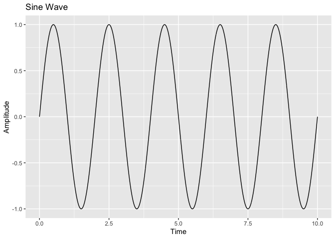
The motion or the velocity of a pendulum can be represented as a time series data. Let’s generate a simple sine wave to illustrate the concept of RQA.
# Generate a sine wave
set.seed(123) # For reproducibility
time_points <- seq(0, 10, by = 0.01)  # Time sequence
sine_wave <- sin(2 * pi * time_points*0.5)  # Sine wave: sin(2*pi*w*t)
cos_wave <- cos(2 * pi * time_points)  # Cosine wave

sin_cos_df <- data.frame(time = time_points, sine_wave = sine_wave, cos_wave = cos_wave)

# Plot the sine wave
ggplot(sin_cos_df, aes(x = time, y = sine_wave)) +
  geom_line() +
  labs(
    title = "Sine Wave",
    x = "Time",
    y = "Amplitude"
  )
# plot time point index vs sine wave
# Add an index column to the dataframe
sin_cos_df$index <- seq_along(sin_cos_df$time)

# Plot time point index vs sine wave
ggplot(sin_cos_df, aes(x = index, y = sine_wave)) +
  geom_line() +
  labs(
    title = "Sine Wave with Time Point Index",
    x = "Index",
    y = "Amplitude"
  ) +
  scale_x_continuous(breaks = seq(0, max(sin_cos_df$index), by = 50))  # Adjust the 'by' value to control density
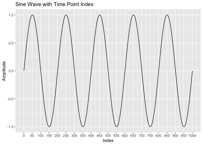
The plot above shows a simple sine wave with a frequency of 1 Hz. The sine wave oscillates between -1 and 1 over a period of 10 seconds. This time series data can be analyzed using RQA to quantify the degree of recurrence in the data. Let’s perform RQA on the sine wave data.
Performing RQA on Sine Wave
Now, we will perform RQA on the sine wave data to quantify the degree of recurrence in the data. We will use the rqa function from the nonlinearTseries package in R to perform RQA. The rqa function requires the following parameters:
embed <- 1  # Embedding dimension
delay <- 5  # Time delay

rqa_result <- nonlinearTseries::rqa(time.series = sine_wave,
                                    embedding.dim = embed,
                                    time.lag = delay,
                                    radius = 0.1,
                                    lmin = 2,
                                    vmin = 2,
                                    do.plot = T)
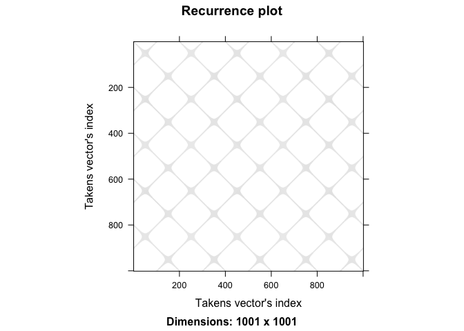
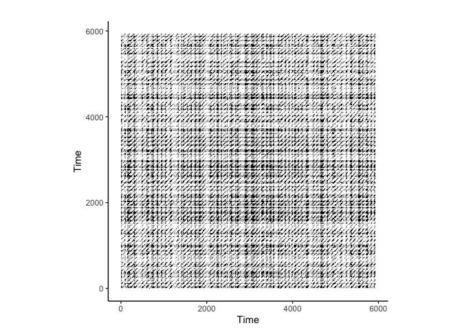
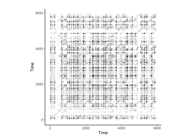
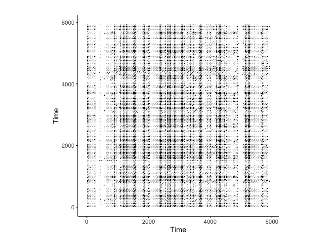
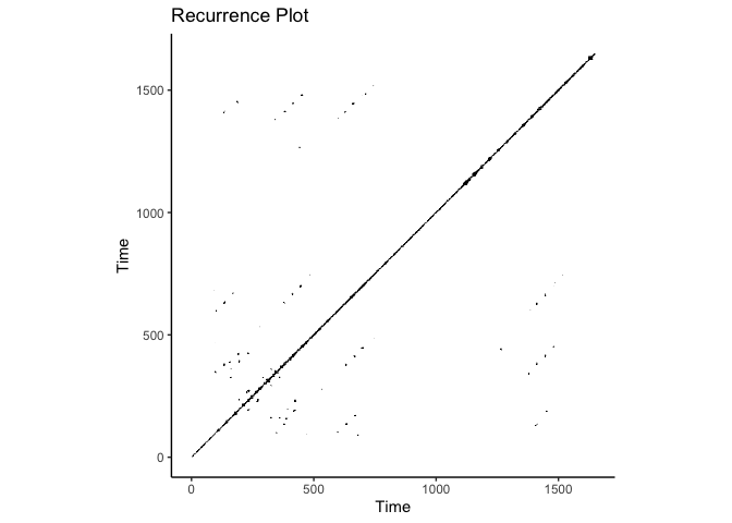
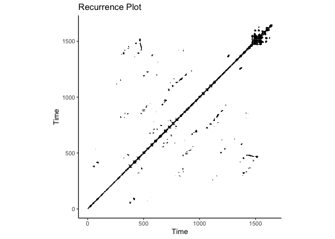
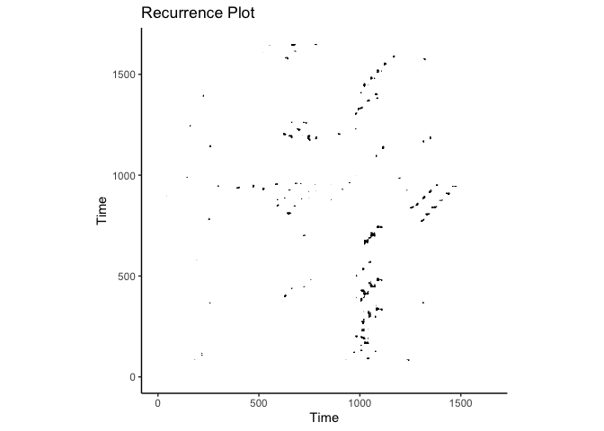
The diagonal lines in the recurrence plot represent recurrent states in the phase space, indicating that the system returns to similar states over time or the two time series are similar. The vertical lines represent the duration of recurrent states, indicating how long the system remains in a particular state. Finally, we quantify this plot using measures like determinism, entropy, and percentage of recurrence. We will talk about these measures in detail in subsequent sections.
crqa is another popular R package perform Cross-Recurrence Quantification Analysis (CRQA), which is an extension of RQA to analyze the recurrence between two time series (we will talk about this in later section). We can compute RQA using the crqa function from the crqa package by providing the same time series twice as input for both ts1 and ts2 arguments.
embed <- 1  # Embedding dimension
delay <- 5  # Time delay

# Perform RQA on the sine wave
rqa_result <- crqa::crqa(
  ts1 = sine_wave,
  ts2 = sine_wave,
  embed = embed,
  delay = delay,
  radius = 0.1,   # Threshold distance for recurrence
  normalize = 1,  # Normalize data
  mindiagline = 2, # Minimum length of diagonal lines
  minvertline = 2, # Minimum length of vertical lines
  whiteline = FALSE
)

# Print RQA results
print(rqa_result[1:9])
## $RR
## [1] 18.96315
##
## $DET
## [1] 99.9779
##
## $NRLINE
## [1] 9569
##
## $maxL
## [1] 1001
##
## $L
## [1] 19.85254
##
## $ENTR
## [1] 2.901428
##
## $rENTR
## [1] 0.6416549
##
## $LAM
## [1] 99.98947
##
## $TT
## [1] 23.53996
crqa::plot_rp(rqa_result$RP)
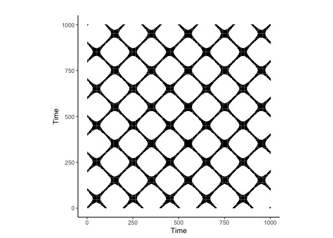
Notice that the plot made using nonlinearTseries::rqa has the y-axis flipped compared to the this crqa::crqa plot. This is because the rqa function in the nonlinearTseries package uses a different convention for the recurrence plot. The diagonal lines in the recurrence plot represent recurrent states in the phase space, indicating that the system returns to similar states over time or the two time series are similar. If you flip back the y-axis, you will see that the two recurrence plots are identical.
Making sense of the paramters
Embedding dimension
Embedding dimension (embed): The number of dimensions in the phase space to embed the time series data. It is used to reconstruct the phase space from the time series data. You may be wondering why we need to embed the time series data in a higher-dimensional space. This is because the dynamics of the system are often governed by multiple variables or factors that interact with each other. Embedding the time series data in a higher-dimensional space allows us to capture these interactions and reconstruct the underlying dynamics of the system.
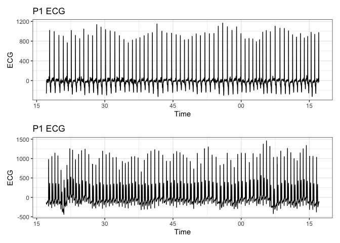
Departure from one-dimensional analysis (Webber Jr & Zbilut, 2005) provides a comprehensive overview of RQA, and I highly recommend reading it. Then analysis of a single time series data as shown above is inherently one-dimensional, the measured quantity itself being a single variable. However, (Wallot & Leonardi, 2018) argue that many behavioral phenomena are inherently multi-dimensional. For example (borrowed from (Wallot, 2019)), consider the Electrocardiogram (ECG) data, which captures the electrical activity of the heart using two electrodes placed on the chest. This setup is essentailly capturing data in one plane (i.e. instead of the three bodily planes: frontal, sagittal, and transverse), and the inherent ECG data is an aggregation of multiple sources at its core.
One question that arises now is, how do we capture the multi-dimensional nature of the data? One way to do this is to use the concept of time-delayed embedding. Takens theorem states that a time-delayed embedding of a time series can recover the underlying dynamics of the system. The theorem states that a time series can be reconstructed from a single variable by using a time-delayed embedding. The time-delayed embedding is a method to reconstruct the phase space of a dynamical system from a single time series.
We can compute the embedding dimension using the false nearest neighbors method. The false nearest neighbors method involves iteratively increasing the embedding dimension and calculating the fraction of false nearest neighbors to determine the optimal embedding dimension. The optimal embedding dimension is the smallest embedding dimension that captures the underlying dynamics of the system.
Time delay
Time delay (delay): The time delay between the embedded time series data points. It is used to reconstruct the phase space from the time series data. The time delay is crucial for capturing the dynamics of the system and is often determined using the autocorrelation function of the time series data. The time delay helps in capturing the temporal structure of the system and is essential for reconstructing the phase space from the time series data. Autocorrelation is a measure of the correlation between the time series data and its lagged values.
Radius
Radius (radius): The threshold distance for recurrence. Maximum distance between two phase-space points to be considered a recurrence. In simple terms, it defines how close two points in the phase space need to be to be considered recurrent.
Making sense of the metrics
Recurrence quantification analysis (RQA) provides several metrics to quantify the degree of recurrence in the data. It is important to understand what they represent and how they can be interpreted.
Recurrence rate
Recurrence rate (RR): The percentage of recurrent points in the phase space within a certain threshold distance. It quantifies the density of recurrence points in a recurrence plot. In other words, it measures how often states in a dynamical system recur over time.
In real sense, the recurrence rate can be altered by changing the threshold distance for recurrence. A higher threshold distance will result in a lower recurrence rate, as the system needs to be closer to be considered recurrent.
What does a high recurrence rate mean in physiological data? A high determinism in physiological data indicates that the system exhibits predictable and structured behavior, with recurring patterns that are sustained over time. This suggests a degree of regularity or coordination in the underlying physiological processes.
Determinism
Determinism (DET): The percentage of recurrent points that form diagonal lines in the recurrence plot. It represents the predictability or regularity of the system. A higher determinism indicates that the system returns to similar states over time and exhibits regular behavior, while a lower determinism indicates that the system explores different states and exhibits irregular behavior. Determinism is a measure of the predictability or regularity of the system.
Determinism (DET) goes a step further - it tells you about the predictability and structure in your system: - DET measures the percentage of recurrent points that form diagonal lines in your recurrence plot - These diagonal lines are crucial because they indicate that segments of your trajectory are running parallel to other segments i.e. the system is revisiting similar states over time
What does a high determinism mean in physiological data? A high determinism in physiological data indicates that the system exhibits predictable and structured behavior, with recurring patterns that are sustained over time. This suggests a degree of regularity or coordination in the underlying physiological processes.
Entropy
Entropy (ENT): The Shannon entropy of the diagonal line lengths in the recurrence plot. It quantifies the complexity or randomness of the system. A higher entropy indicates that the system explores a wide range of states and exhibits complex behavior, while a lower entropy indicates that the system returns to similar states and exhibits regular behavior. Entropy is a measure of the complexity or randomness of the system.
Embedding dimension greater than 1
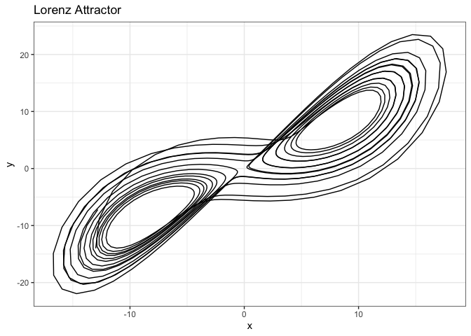
We will now look at another example - Lorenz attractor - to demonstrate the importance of embedding dimension greater than 1. This is a set of three coupled differential equations that describe the trajectory of a particle moving in a three-dimensional space with equations:
\begin{equation} \frac{dx}{dt} = \sigma(y - x) \end{equation}
\begin{equation} \frac{dy}{dt} = x(\rho - z) - y \end{equation}
\begin{equation} \frac{dz}{dt} = xy - \beta z \end{equation}
where \(x\), \(y\), and \(z\) are the state variables, and \(\sigma\), \(\rho\), and \(\beta\) are the system parameters. The Lorenz attractor exhibits chaotic behavior, and the trajectory of the particle in the phase space is sensitive to the initial conditions.
We will generate the time series data for the Lorenz attractor and perform RQA on it. We will assume that we are only able to observe the \(x\) variable and use it as the time series data. We will embed the time series data in a three-dimensional space (or more) and perform RQA on it.
This example is borrowed from (Wallot & Leonardi, 2018), an excellent resource for understanding the application of CRQA.
lorData <- nonlinearTseries::lorenz(time = seq(0, 20, by = 0.02), do.plot = T)
# head(lorData)

lorData <- as.data.frame(lorData)

ggplot(lorData, aes(x = x, y = y, z = z)) +
  geom_path() +
  labs(title = "Lorenz Attractor", x = "x", y = "y", z = "z") +
  theme_bw()
# Plotly plot
p<- plot_ly(lorData,
        x = ~x,
        y = ~y,
        z = ~z,
        type = 'scatter3d',
        mode = 'lines',
        line = list(width = 2, color = ~z, colorscale = 'Viridis')) %>%
  layout(
    title = "Lorenz Attractor",
    scene = list(
      camera = list(
        eye = list(x = 1.5, y = 1.5, z = 1.5)
      ),
      aspectmode = "data",
      xaxis = list(title = "X"),
      yaxis = list(title = "Y"),
      zaxis = list(title = "Z")
    )
  )

p
Average mutual information
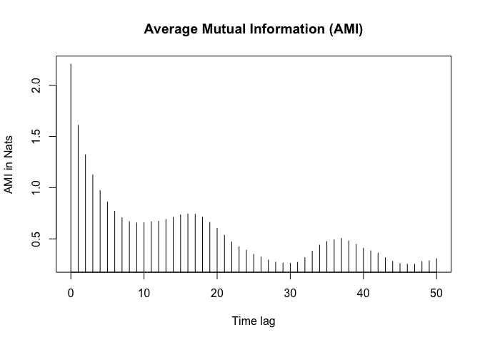
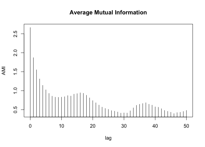
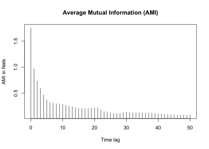
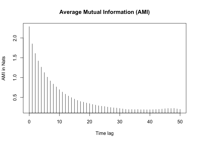
The average mutual information (AMI) captures the amount of information shared between two points in the phase space as a function of the time delay. The AMI is used to determine the optimal time delay for a time series data. The optimal time delay is the time delay that captures the underlying dynamics of the system and is often determined using the first local minimum of the AMI curve.
# Compute AMI
ami_values <- nonlinearTseries::mutualInformation(lorData$x,
                                                  lag.max = 50,
                                                  do.plot = T)
amis <- ami_values$mutual.information
# plot(1:51, amis, type = "l", xlab = "Lag", ylab = "AMI", main = "Lag vs AMI")

# fist local minima
delay <- which(diff(sign(diff(amis))) == 2) + 1
delay <- delay[1]
delay
## [1] 10
# can also be computed using tseriesChaos package
ami_values <- tseriesChaos::mutual(lorData$x, lag.max = 50)
min_index <- which.min(ami_values)
min_value <- ami_values[min_index]
min_index
## 46
## 47
False Nearest Neighbors
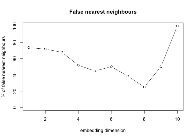
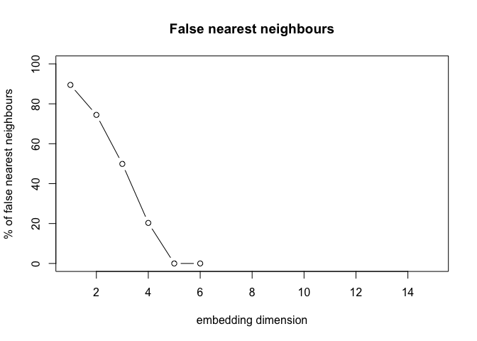
The false nearest neighbors (FNN) method is used to determine the minimum embedding dimension for a time series data. The FNN method involves iteratively increasing the embedding dimension and calculating the fraction of false nearest neighbors to determine the optimal embedding dimension. The optimal embedding dimension is the smallest embedding dimension that captures the underlying dynamics of the system. It is advised to overestimate the time delay to avoid missing the underlying dynamics of the system.
# Compute FNN
fnn_values <- tseriesChaos::false.nearest(lorData$x,
                                         m = 20, # maximum embedding dimension (search param)
                                         d=delay, # time delay
                                         t=0 # theiler window
                                         )

# plot the FNN values
tseriesChaos::plot.false.nearest(fnn_values)

# Extract the 'fraction' row
fraction_values <- fnn_values["fraction", ]

# Convert to numeric, removing empty values (if any)
fraction_values <- as.numeric(fraction_values[!is.na(fraction_values)])

# Find the first local minimum index in the FNN values
embed_dim <- which(diff(sign(diff(fraction_values))) > 0) + 1
embed_dim <- embed_dim[1]
embed_dim
## [1] 4
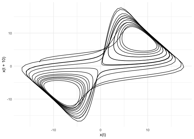
The minima is at embedding dimension 4 but since the curve flattens out at 3 and for easy visualization, we will use embedding dimension 3 (ideally 4 - the higher should be chosen when in doubt).
On a side note, Theiler window is a temporal window that limits the number of nearby data points that are used in the False Nearest Neighbors (FNN) analysis. The purpose of this window is to ensure that when you’re checking for false nearest neighbors, you avoid using data points that are too close in time to one another, as these could be highly autocorrelated and therefore not valid for the analysis. Essentially, it’s a way to exclude points that are too similar due to being in close proximity in time, and this helps to improve the robustness of the analysis.
Phase Space Reconstruction
Phase-space reconstruction through 3-D embedding of the individual time-series
# define x1, x2, x3 using delay
x1 <- lorData$x[1:(length(lorData$x) - 2 * delay)]  # x(t)
x2 <- lorData$x[(1 +  delay):(length(lorData$x) -  delay)]  # x(t + delay)
x3 <- lorData$x[(1 + 2 * delay):length(lorData$x)]  # x(t + 2 x delay)

new_data <- data.frame(x1=x1,
                       x2=x2,
                       x3=x3)

ggplot(new_data, aes(x = x1, y = x2)) +
  geom_path() +
  labs(title = NULL, x = "x(t)", y = "x(t + 10)") +
  theme_minimal()
p<- plot_ly(new_data,
        x = ~x1,
        y = ~x2,
        z = ~x3,
        type = 'scatter3d',
        mode = 'lines',
        line = list(width = 2, color = ~x3, colorscale = 'Viridis')) %>%
  layout(
    title = "Lorenz Attractor",
    scene = list(
      camera = list(
        eye = list(x = 1.5, y = 1.5, z = 1.5)
      ),
      aspectmode = "data",
      xaxis = list(title = "X"),
      yaxis = list(title = "Y"),
      zaxis = list(title = "Z")
    )
  )

p
# embed using lorData$x
x1 <- lorData$x[1:(length(lorData$x) - 2 * delay)]
x2 <- lorData$x[(1 +  delay):(length(lorData$x) -  delay)]
x3 <- lorData$x[(1 + 2 * delay):length(lorData$x)]

# embed using lorData$y
y1 <- lorData$y[1:(length(lorData$y) - 2 * delay)]
y2 <- lorData$y[(1 +  delay):(length(lorData$y) -  delay)]
y3 <- lorData$y[(1 + 2 * delay):length(lorData$y)]

new_data <- data.frame(x1=x1,
                       x2=x2,
                       x3=x3,
                       y1=y1,
                       y2=y2,
                       y3=y3)

# Define the two traces for xx, xy, xz
trace1 <- plot_ly(
  new_data,
  x = ~x1,
  y = ~x2,
  z = ~x3,
  type = 'scatter3d',
  mode = 'lines',
  line = list(width = 2, color = 'blue')
) %>%
  layout(scene = list(
    xaxis = list(title = "X(t)"),
    yaxis = list(title = "X(t + 10)"),
    zaxis = list(title = "X(t + 19)"),
    aspectmode = "data"
  ))

# Define the two traces for yx, yy, yz
trace2 <- plot_ly(
  new_data,
  x = ~y1,
  y = ~y2,
  z = ~y3,
  type = 'scatter3d',
  mode = 'lines',
  line = list(width = 2, color = 'red')
) %>%
  layout(scene = list(
    xaxis = list(title = "Y(t)"),
    yaxis = list(title = "Y(t + 10)"),
    zaxis = list(title = "Y(t + 19)"),
    aspectmode = "data"
  ))

# Combine the plots into one visualization using subplot
p<-subplot(
  trace1, trace2,
  nrows = 1,  # Arrange plots in one row
  titleX = TRUE, titleY = TRUE, shareY = FALSE
) %>%
  layout(title = "Two Delayed Plots")

p
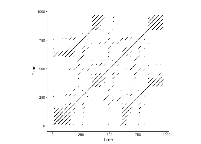
RQA on Lorenz Attractor
RQA with multidimensional embedding
# Perform RQA on the Lorenz attractor
rqa_result <- crqa::crqa(
  ts1 = lorData$x,
  ts2 = lorData$x,
  embed = embed_dim,
  delay = delay,
  radius = 0.1,   # Threshold distance for recurrence
  normalize = 1,  # Normalize data
  mindiagline = 2, # Minimum length of diagonal lines
  minvertline = 2, # Minimum length of vertical lines
  tw = 0,         # Theiler window
  whiteline = FALSE,
  side = "both"
)

# Print RQA results
print(rqa_result[1:9])
## $RR
## [1] 2.348752
##
## $DET
## [1] 99.06977
##
## $NRLINE
## [1] 1741
##
## $maxL
## [1] 971
##
## $L
## [1] 12.60138
##
## $ENTR
## [1] 2.882162
##
## $rENTR
## [1] 0.6761384
##
## $LAM
## [1] 98.60917
##
## $TT
## [1] 4.086265
# plot
crqa::plot_rp(rqa_result$RP)
CRQA on Lorenz Attractor
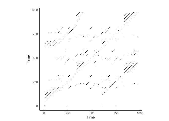
Notice we only change the ts2 to lorData$y to perform CRQA
# Perform RQA on the Lorenz attractor
rqa_result <- crqa::crqa(
  ts1 = lorData$x,
  ts2 = lorData$y,
  embed = embed_dim,
  delay = delay,
  radius = 0.1,   # Threshold distance for recurrence
  normalize = 1,  # Normalize data
  mindiagline = 2, # Minimum length of diagonal lines
  minvertline = 2, # Minimum length of vertical lines
  tw = 0,         # Theiler window
  whiteline = FALSE,
  side = "both"
)

# Print RQA results
print(rqa_result[1:9])
## $RR
## [1] 0.6662841
##
## $DET
## [1] 96.19548
##
## $NRLINE
## [1] 1200
##
## $maxL
## [1] 38
##
## $L
## [1] 5.035833
##
## $ENTR
## [1] 2.178686
##
## $rENTR
## [1] 0.634448
##
## $LAM
## [1] 87.88602
##
## $TT
## [1] 2.8154
# plot
crqa::plot_rp(rqa_result$RP)
Electrocardiogram (ECG) Data Analysis
# load csv file with headers
ecg_data <-  read_csv("ecg.csv")
## New names:
## Rows: 184771 Columns: 10
## ── Column specification
## ──────────────────────────────────────────────────────── Delimiter: "," chr
## (3): eid, p1_id, p2_id dbl (6): ...1, p1_ecg, p2_ecg, trial, condition,
## local_trial dttm (1): timestamp
## ℹ Use `spec()` to retrieve the full column specification for this data. ℹ
## Specify the column types or set `show_col_types = FALSE` to quiet this message.
## • `` -> `...1`
# convert timestamp to POSIXct
ecg_data$timestamp <- as.POSIXct(ecg_data$timestamp, format = "%Y-%m-%d %H:%M:%OS")

# Convert data to a tsibble object
ecg_tsibble <- ecg_data %>%
  as_tsibble(index = timestamp)

# Resample to 100 Hz using interval = "0.01 secs"
ecg_resampled <- ecg_tsibble %>%
  index_by(new_time = ~ floor_date(.x, "0.01 secs")) %>% # Adjust timestamp to nearest 10ms
  summarize(p1_ecg = mean(p1_ecg, na.rm = TRUE),
            p2_ecg = mean(p2_ecg, na.rm = TRUE)
            ) # Use mean for downsampling

# subset data
ecg_resampled <- ecg_resampled[4000:10000,]

# plot p1_ecg
p1<-ecg_resampled %>%
  ggplot(aes(x = new_time, y = p1_ecg)) +
  geom_line() +
  labs(title = "P1 ECG", x = "Time", y = "ECG") +
  theme_bw()

# plot p1_ecg
p2<-ecg_resampled %>%
  ggplot(aes(x = new_time, y = p2_ecg)) +
  geom_line() +
  labs(title = "P1 ECG", x = "Time", y = "ECG") +
  theme_bw()


p1 / p2
# Add an index column to the data for plotting
ecg_resampled_ <- ecg_resampled %>%
  mutate(index = row_number())


# Plot using the new index
p1_ <- ecg_resampled_ %>%
  ggplot(aes(x = index, y = p1_ecg)) +
  geom_line() +
  labs(title = "P1 ECG", x = "Index", y = "ECG") +
  theme_bw()

p2_ <- ecg_resampled_ %>%
  ggplot(aes(x = index, y = p2_ecg)) +
  geom_line() +
  labs(title = "P1 ECG", x = "Index", y = "ECG") +
  theme_bw()

p1_ / p2_
AMI on ECG Data
# Compute AMI
ami_values <- nonlinearTseries::mutualInformation(ecg_resampled$p2_ecg,
                                                  lag.max = 50,
                                                  do.plot = T)
amis <- ami_values$mutual.information
# plot(1:21, amis, type = "l", xlab = "Lag", ylab = "AMI", main = "AMI vs Lag")

# fist local minima
delay <- which(diff(sign(diff(amis))) == 2) + 1
delay <- delay[1]
delay
## [1] 18
FNN on ECG Data
# Compute FNN
fnn_values <- tseriesChaos::false.nearest(ecg_resampled$p2_ecg,
                                         m = 10,
                                         d=delay,
                                         t=1
                                         )

# plot the FNN values
tseriesChaos::plot.false.nearest(fnn_values)
# Extract the 'fraction' row
fraction_values <- fnn_values["fraction", ]

# Convert to numeric, removing empty values (if any)
fraction_values <- as.numeric(fraction_values[!is.na(fraction_values)])

# Find the first local minimum index in the FNN values
embed_dim <- which(diff(sign(diff(fraction_values))) > 0) + 1
embed_dim <- embed_dim[1]
embed_dim
## [1] 5
RQA on ECG Data
# Perform RQA on the ecg data
rqa_result <- crqa::crqa(
  ts1 = ecg_resampled$p1_ecg,
  ts2 = ecg_resampled$p1_ecg,
  embed = embed_dim,
  delay = delay,
  radius = 0.1,   # Threshold distance for recurrence
  normalize = 1,  # Normalize data
  mindiagline = 2, # Minimum length of diagonal lines
  minvertline = 2, # Minimum length of vertical lines
  tw = 0,         # Theiler window
  whiteline = FALSE,
  side = "both"
)

print(rqa_result[1:9])
## $RR
## [1] 16.68069
##
## $DET
## [1] 92.8737
##
## $NRLINE
## [1] 1173703
##
## $maxL
## [1] 5929
##
## $L
## [1] 4.639929
##
## $ENTR
## [1] 2.11479
##
## $rENTR
## [1] 0.4402126
##
## $LAM
## [1] 95.89235
##
## $TT
## [1] 6.376579
# plot
crqa::plot_rp(rqa_result$RP)
# Perform RQA on the ecg data
rqa_result <- crqa::crqa(
  ts1 = ecg_resampled$p2_ecg,
  ts2 = ecg_resampled$p2_ecg,
  embed = embed_dim,
  delay = delay,
  radius = 0.1,   # Threshold distance for recurrence
  normalize = 1,  # Normalize data
  mindiagline = 2, # Minimum length of diagonal lines
  minvertline = 2, # Minimum length of vertical lines
  tw = 0,         # Theiler window
  whiteline = FALSE,
  side = "both"
)

print(rqa_result[1:9])
## $RR
## [1] 6.827498
##
## $DET
## [1] 86.51108
##
## $NRLINE
## [1] 557649
##
## $maxL
## [1] 5929
##
## $L
## [1] 3.723362
##
## $ENTR
## [1] 1.716389
##
## $rENTR
## [1] 0.3894937
##
## $LAM
## [1] 93.21525
##
## $TT
## [1] 4.523905
# plot
crqa::plot_rp(rqa_result$RP)
CRQA on ECG Data
# Perform RQA on the ecg data
rqa_result <- crqa::crqa(
  ts1 = ecg_resampled$p1_ecg,
  ts2 = ecg_resampled$p2_ecg,
  embed = embed_dim,
  delay = delay,
  radius = 0.1,   # Threshold distance for recurrence
  normalize = 1,  # Normalize data
  mindiagline = 2, # Minimum length of diagonal lines
  minvertline = 2, # Minimum length of vertical lines
  tw = 0,         # Theiler window
  whiteline = FALSE,
  side = "both"
)

print(rqa_result[1:9])
## $RR
## [1] 8.610749
##
## $DET
## [1] 87.73045
##
## $NRLINE
## [1] 710177
##
## $maxL
## [1] 12
##
## $L
## [1] 3.739276
##
## $ENTR
## [1] 1.750265
##
## $rENTR
## [1] 0.7299173
##
## $LAM
## [1] 95.15887
##
## $TT
## [1] 4.84185
# plot
crqa::plot_rp(rqa_result$RP)
Interbeat Interval Data Analysis
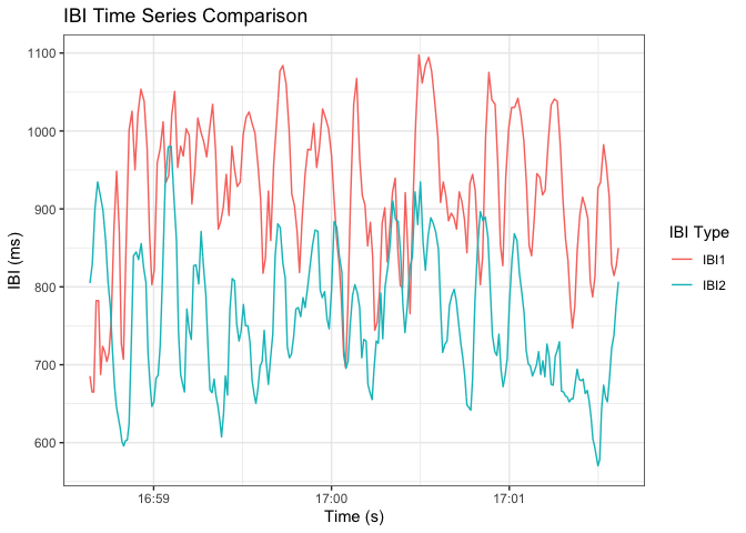
Note: the data used here is preprocess after appropriate resampling such that we have IBI data for each participant at any given time.
ibi_data <- read.csv("ibi.csv") # time, IBI1, IBI2

# convert time format 2023-06-29 16:06:08.409180
ibi_data$time <- as.POSIXct(ibi_data$time, format = "%Y-%m-%d %H:%M:%OS")

# plot IBI time series
# Reshape the data to a long format
ibi_long <- ibi_data %>%
  pivot_longer(cols = c(IBI1, IBI2), names_to = "IBI_type", values_to = "IBI_value")

# Plot both IBI1 and IBI2 in one plot
ggplot(ibi_long, aes(x = time, y = IBI_value, color = IBI_type)) +
  geom_line() +
  labs(title = "IBI Time Series Comparison", x = "Time (s)", y = "IBI (ms)", color = "IBI Type") +
  theme_bw()
AMI on IBI Data
AMI = Auto Mutual Information AMI is used to determine the time delay for a time series.
# Compute AMI
ami_values <- nonlinearTseries::mutualInformation(ibi_data$IBI2,
                                                  lag.max = 50,
                                                  do.plot = T)
# Compute the first minimum of AMI
amis <- ami_values$mutual.information

# fist local minima
delay <- which(diff(sign(diff(amis))) == 2) + 1
delay <- delay[1]
delay
## [1] 34
FNN on IBI Data
FNN is used to determine the minimum embedding dimension for a time series.
# Compute FNN
fnn_values <- tseriesChaos::false.nearest(ibi_data$IBI1,
                                         m = 15,
                                         d=delay,
                                         t=1
                                         )

# plot the FNN values
tseriesChaos::plot.false.nearest(fnn_values)
# Extract the 'fraction' row
fraction_values <- fnn_values["fraction", ]

# Convert to numeric, removing empty values (if any)
fraction_values <- as.numeric(fraction_values[!is.na(fraction_values)])

# Find the first local minimum index in the FNN values
embed_dim <- which(diff(sign(diff(fraction_values))) > 0) + 1
embed_dim <- embed_dim[1]
embed_dim
## [1] 5
RQA on IBI Data
rqa_res = crqa::crqa(
  ts1 = ibi_data$IBI1,
  ts2 = ibi_data$IBI1,
  embed = embed_dim,
  delay = delay,
  radius = 0.1,   # Threshold distance for recurrence
  normalize = 1,  # Normalize data
  mindiagline = 2, # Minimum length of diagonal lines
  minvertline = 2, # Minimum length of vertical lines
  tw = 0,         # Theiler window
  whiteline = FALSE,
  side = "both"
)

# Print RQA results
print(rqa_res[1:9])
## $RR
## [1] 0.5278537
##
## $DET
## [1] 98.91183
##
## $NRLINE
## [1] 991
##
## $maxL
## [1] 1648
##
## $L
## [1] 14.30878
##
## $ENTR
## [1] 2.408787
##
## $rENTR
## [1] 0.6670843
##
## $LAM
## [1] 99.65123
##
## $TT
## [1] 7.027054
crqa::plot_rp(rqa_res$RP, title = "Recurrence Plot")
rqa_res = crqa::crqa(
  ts1 = ibi_data$IBI2,
  ts2 = ibi_data$IBI2,
  embed = embed_dim,
  delay = delay,
  radius = 0.2,   # Threshold distance for recurrence
  normalize = 1,  # Normalize data
  mindiagline = 2, # Minimum length of diagonal lines
  minvertline = 2, # Minimum length of vertical lines
  tw = 0,         # Theiler window
  whiteline = FALSE,
  side = "both"
)

# Print RQA results
print(rqa_res[1:9])
## $RR
## [1] 1.849624
##
## $DET
## [1] 99.65362
##
## $NRLINE
## [1] 3409
##
## $maxL
## [1] 1648
##
## $L
## [1] 14.68466
##
## $ENTR
## [1] 2.974163
##
## $rENTR
## [1] 0.7178534
##
## $LAM
## [1] 99.85269
##
## $TT
## [1] 15.18619
crqa::plot_rp(rqa_res$RP, title = "Recurrence Plot")
CRQA on IBI Data
rqa_res = crqa::crqa(
  ts1 = ibi_data$IBI1,
  ts2 = ibi_data$IBI2,
  embed = embed_dim,
  delay = delay,
  radius = 0.2,   # Threshold distance for recurrence
  normalize = 1,  # Normalize data
  mindiagline = 2, # Minimum length of diagonal lines
  minvertline = 2, # Minimum length of vertical lines
  tw = 0,         # Theiler window
  whiteline = FALSE,
  side = "both"
)

# Print RQA results
print(rqa_res[1:9])
## $RR
## [1] 0.3534366
##
## $DET
## [1] 98.63527
##
## $NRLINE
## [1] 1590
##
## $maxL
## [1] 31
##
## $L
## [1] 5.954717
##
## $ENTR
## [1] 2.360008
##
## $rENTR
## [1] 0.7331776
##
## $LAM
## [1] 99.30201
##
## $TT
## [1] 8.571942
crqa::plot_rp(rqa_res$RP, title = "Recurrence Plot")
Multi-dimensional RQA (MdRQA)
Why do we need a multi-dimensional extension of RQA? Increasingly behaviorial analysis is capturing physiological data such as heart rate, respiration, and dermal activity. These data streams are often interdependent, reflecting the complex interactions between physiological and psychological processes. Traditional RQA is limited to analyzing a single time series, making it difficult to capture the rich dynamics of multi-dimensional data. Multi-dimensional RQA (MdRQA) extends the RQA framework to analyze the similarity between multiple time series, offering a more nuanced understanding of complex behavioral interactions.
(Wallot, 2019) provides a comprehensive overview of MdRQA, and I highly recommend reading it. In the next section, we will discuss the basic idea behind MdRQA and how it can be used to analyze multi-dimensional data.
https://github.com/Wallot/MdRQA
Multi-dimensional CRQA (MdCRQA)
Multi-dimensional CRQA (MdCRQA) extends the CRQA framework to analyze the similarity between multiple time series. MdCRQA is a tool for studying the complex interactions between physiological and psychological processes, providing insights into the dynamics of multi-dimensional data.
https://github.com/Wallot/MdCRQA
Conclusion
In this post, we discussed the basics of Recurrence Quantification Analysis (RQA) and its application to physiological data. We covered the key concepts of RQA, including Recurrence Rate (RR), Determinism (DET), and Entropy (ENT), and demonstrated how to perform RQA on different types of physiological data, including the Lorenz attractor, electrocardiogram (ECG) data, and interbeat interval (IBI) data. We also discussed the importance of embedding dimension and time delay in RQA and how to determine these parameters using the Average Mutual Information (AMI) and False Nearest Neighbors (FNN) methods.
MdRQA and MdCRQA will be covered in a separate post soon. A lot of the content in this post is inspired and sometimes directly borrowed from the excellent resources (Carello & Moreno, 2005; Webber Jr & Zbilut, 2005; Wallot, 2019; Wallot & Leonardi, 2018; Eloy et al., 2023). I highly recommend reading them for a deeper understanding of the concepts discussed here.
References
2023
- Capturing the Dynamics of Trust and Team Processes in Human-Human-Agent Teams via Multidimensional Neural Recurrence AnalysesProceedings of the ACM on Human-Computer Interaction, 2023
2019
- Multidimensional Cross-Recurrence Quantification Analysis (MdCRQA)–a method for quantifying correlation between multivariate time-seriesMultivariate behavioral research, 2019
2018
- Analyzing multivariate dynamics using cross-recurrence quantification analysis (crqa), diagonal-cross-recurrence profiles (dcrp), and multidimensional recurrence quantification analysis (mdrqa)–a tutorial in rFrontiers in psychology, 2018
2005
- Why nonlinear methodsTutorials in contemporary nonlinear methods for the behavioral sciences, 2005
- Recurrence quantification analysis of nonlinear dynamical systemsTutorials in contemporary nonlinear methods for the behavioral sciences, 2005
Enjoy Reading This Article?
Here are some more articles you might like to read next: