Preprocessing functional Near Infrared Spectroscopy (fNIRS) Data

Contents

• Introduction
• Raw Data
• Removing noise
  • Motion Artifact Detection and Correction
  • Removing physiological noise
• Convert Optical Density to Concentration
  • Beer-Lambert Law
  • Modified Beer-Lambert Law
• Feature Extraction and Averaging

Introduction

Functional Near Infrared Spectroscopy (fNIRS) is a non-invasive brain imaging technique that measures the changes in the concentration of oxyhemoglobin and deoxyhemoglobin in the brain. The way it works is by shining near-infrared light through the skull and into the brain tissue. This light is absorbed differently by oxygenated and deoxygenated hemoglobin, allowing researchers to infer changes in blood flow and oxygenation in specific brain regions.

fNIRS is particularly useful for studying brain activity in naturalistic settings, as it is portable and can be used with participants who are moving or engaged in various activities. However, like any other neuroimaging technique, fNIRS data requires careful preprocessing to ensure that the signals are clean and interpretable. Broadly speaking, fNIRS has better spatial resolution than EEG but lower temporal resolution. I recommend reading the Mehta et al. (2023) (Mehta & Parasuraman, 2013) paper for a more detailed comparison of fNIRS with other neuroimaging techniques like EEG, fMRI, and MEG.

flowchart TD
    A[Raw Light Intensity Signal] --> C[Convert to Optical Density]
    
    C --> E[Motion Artifact Detection]
    E --> F[Motion Correction]
    F --> G[Bandpass Filter]
    
    G --> G1[Heartbeat<br/>~1-2 Hz]
    G --> G2[Respiration<br/>~0.4 Hz]
    G --> G3[Mayer Waves<br/>Blood Pressure<br/>~0.1 Hz]
    
    G1 --> H[Filtered Signal]
    G2 --> H
    G3 --> H
    
    H --> I[Convert Optical Density<br/>to Concentration]
    I --> J[Feature Extraction & Averaging]
    
    J --> K1[HbO max]
    J --> K2[HbO mean]
    J --> K3[Connectivity Measures]
    J --> K4[Other Features]
    
    K1 --> L[Statistical Analysis]
    K2 --> L
    K3 --> L
    K4 --> L

Note:

• fNIRS and EEG are more portable and suitable for naturalistic or pediatric studies.
• fMRI and MEG offer higher spatial resolution but are less portable and more expensive.

Raw Data

The raw data from fNIRS is light intensity signals recorded from the scalp. These signals are typically collected from multiple channels, each corresponding to a specific location on the head.

Typically, the recording is done with two different wavelengths of light (usually around 690 nm and 830 nm), which allows for the measurement of the signals from oxyhemoglobin and deoxyhemoglobin.

The light intensity is converted to optical density (OD) using the following formula:

\[OD = -\log_{10}\left(\frac{I_1}{I_0}\right) = \log\left(\frac{I_0}{I_1}\right)\]

where \(I_1\) is the intensity of the light received by the detector and \(I_0\) is the intensity of the light emitted by the source.

Removing noise

The raw fNIRS data is often contaminated with noise from various sources, including motion artifacts, physiological signals (like heartbeat and respiration), and environmental noise. To clean the data, several preprocessing steps are typically applied.

Motion Artifact Detection and Correction

Motion artifacts are one of the most significant sources of noise in fNIRS data. They can arise from head movements, muscle contractions, or other physical activities during the recording. To detect and correct for motion artifacts, several methods can be employed.

Some motion correction methods require explicitly identifying the motion artifacts, while others use statistical methods to estimate and remove them. In Homer3, a popular fNIRS data analysis software, the motion artifact detection can be done using the hmrMotionArtifactByChannel function. This function uses a threshold-based approach to identify motion artifacts in the data. Typical parameters for this function include: tMotion=0.5, tMask=2, STDEVthresh=20, AMPthresh=0.5. Another option is to use hmrMotionArtifact function

These are followed by motion correction algorithms, Homer3 provides several options for motion correction, including:

• hmrR_MotionCorrectCbsi: This function implements a motion correction algorithm based on the detected motion artifacts. function data_dc = hmrR_MotionCorrectCbsi(data_dc, mlActAuto, turnon)
• hmrR_MotionCorrectPCA: This function implements a motion correction algorithm using Principal Component Analysis (PCA). [data_d, svs, nSV] = hmrR_MotionCorrectPCA(data_d, mlActMan, mlActAuto, tIncMan, tIncAuto, nSV)

There are several other motion correction algorithms available in Homer3, such as hmrR_MotionCorrectWavelet and hmrR_MotionCorrectSpline. Each of these algorithms has its own strengths and weaknesses, and the choice of algorithm depends on the specific characteristics of the data and the research question being addressed. I highly recommend reading the associated papers for each algorithm for a deeper understanding of performance. I also recommend, playing around with several of these algorithms to see which one works best for your data. Always visualize the results of the motion correction to ensure that the artifacts have been effectively removed.

A lot of these alorithms require the user to manually select the motion artifacts, which can be time-consuming and subjective. However, there are automated methods that can help with this process. One such method is Temporal Derivative Distribution Repair (TDDR) (Fishburn et al., 2019), which is a data-driven approach that uses the temporal derivative of the signal to identify and correct motion artifacts. Currently, TDDR is not implemented in Homer3, Matlab and Python, but it is available in the https://github.com/frankfishburn/TDDR. In addition, it is also implemented in the MNE-Python package, which is a popular Python package for neuroimaging data analysis.

Removing physiological noise

Any signal can be decomposed into its frequency components using Fourier Transform. PSD (Power Spectral Density) can be used to analyze the frequency content of the signal. The PSD can be estimated using various methods, such as Welch’s method (scipy.signal.welch in Python). Sources of physiological noise include heartbeat, respiration, and Mayer waves (which are related to blood pressure fluctuations).

Frequency breakdown of fNIRS signals:

• Heartbeat: ~1-2 Hz
• Respiration: ~0.4 Hz
• Mayer waves (blood pressure): ~0.1 Hz
• Useful fNIRS signals: typically below 0.1 Hz

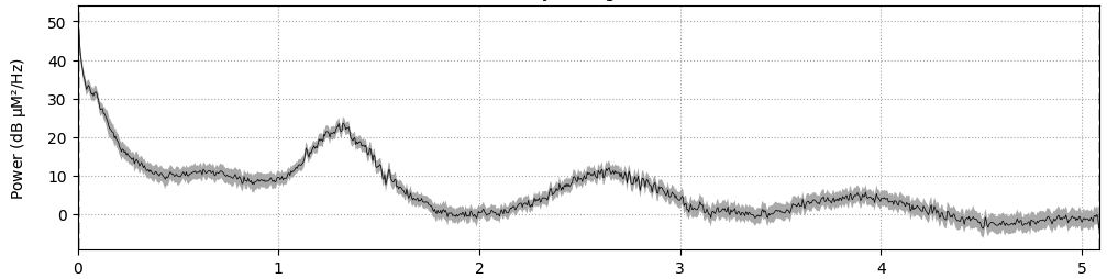
Figure 1: Example Power Spectral Density (PSD) plot of fNIRS data (x-axis is frequency in Hz), illustrating the frequency components corresponding to heartbeat, respiration, Mayer waves, and the low-frequency band of interest.

Bandpass Filtering: A bandpass filter can be applied to isolate the frequency range of interest. Typically, a bandpass filter with a cutoff frequency of 0.01 Hz to 0.5 Hz is used.

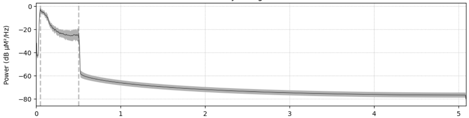
Figure 2: Filtered Power Spectral Density (PSD) plot of fNIRS data (x-axis is frequency in Hz).

Convert Optical Density to Concentration

Once the optical density signals are cleaned, they can be converted to concentration changes of oxyhemoglobin (HbO) and deoxyhemoglobin (HbR) using the modified Beer-Lambert law. This law relates the changes in optical density to the concentration changes of hemoglobin in the brain.

Beer-Lambert Law

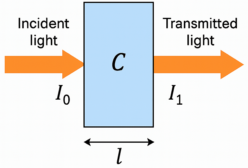
Figure 3: Beer-Lambert Law Diagram, illustrating the relationship between light intensity, optical density, and concentration of absorbing species.

The Beer-Lambert law describes the relationship between the intensity of light absorbed by a substance and its concentration. It is expressed as:

\[OD(\lambda) = \log\left(\frac{I_{0\lambda}}{I_{1\lambda}}\right) = \alpha(\lambda) \cdot c \cdot l\]

where:

• \(OD(\lambda)\) is the optical density at wavelength \(\lambda\)
• \(\alpha(\lambda)\) is the molar extinction coefficient (also called absorption coefficient or specific absorption coefficient) at wavelength \(\lambda\). It quantifies how strongly a particular substance (e.g., HbO\(_2\) or HHb) absorbs light at that wavelength.
• \(c\) is the concentration of the absorbing species (HbO or HbR)
• \(l\) is the path length of the light through the tissue

Modified Beer-Lambert Law

Why modify? The original Beer-Lambert law assumes a clear medium with no scattering, which is not the case in biological tissues. In tissues, light scattering significantly affects the path length of light, so we need to account for this. The modified Beer-Lambert law incorporates a correction factor for scattering, known as the differential path length factor (DPF), and a term for scattering effects, denoted as \(S(\lambda)\) (Baker et al., 2014). The modified Beer-Lambert law is expressed as:

\[OD(\lambda) = \log\left(\frac{I_{0\lambda}}{I_{1\lambda}}\right) = \alpha(\lambda) \cdot c \cdot l \cdot DPF + S(\lambda)\]

where:

• \(OD(\lambda)\) is the optical density at wavelength \(\lambda\)
• \(\alpha(\lambda)\) is the molar extinction coefficient (also called absorption coefficient or specific absorption coefficient) at wavelength \(\lambda\)
• \(c\) is the concentration of the absorbing species (e.g., HbO\(_2\) or HHb)
• \(l\) is the path length of the light through the tissue
• \(DPF\) is the differential path length factor, which accounts for the scattering of light in biological tissues
• \(S(\lambda)\) is a term that accounts for scattering effects and other factors that may affect the light absorption in biological tissues.

For continuous wave (CW) fNIRS, the above equation is typically expressed in terms of changes in optical density, i.e., the difference between two consecutive time points (\(t_n\) and \(t_{n-1}\)):

\[\Delta OD(\lambda) = \alpha(\lambda) \cdot \Delta c \cdot l \cdot DPF\]

Notice the \(S(\lambda)\) term gets cancelled out when calculating the change in optical density.

Partial Volume Factor (PVF): PVF is applied as another correction factor to adjust for the fraction of the path that actually goes through the brain tissue (i.e. excluding scalp, skull, and other tissues).

The equation above now becomes:

\[\Delta OD(\lambda) = \alpha(\lambda) \cdot \Delta c \cdot l \cdot DPF \cdot PVF\]

These correction factors (DPF and PVF) are combined into a single term called the partial pathlength factor (PPF) (Whiteman et al., 2018), which is often used in fNIRS studies:

\[\Delta OD(\lambda) = \alpha(\lambda) \cdot \Delta c \cdot l \cdot PPF\]

where: \(PPF = DPF \cdot PVF\)

Note: all these correction factors are function of wavelength \(\lambda\), so they can be expressed as \(\alpha(\lambda)\), \(DPF(\lambda)\), and \(PVF(\lambda)\).

“Typical value is ~6 for each wavelength if the absorption change is uniform over the volume of tissue measured. To approximate the partial volume effect of a small localized absorption change within an adult human head, this value could be as small as 0.1. Convention is becoming to set ppf=1 and to not divide by the source-detector separation such that the resultant “concentration” is in units of Molar mm (or Molar cm if those are the spatial units). This is becoming wide spread in the literature but there is no fixed citation. Use a value of 1 to choose this option.” - hmrR_OD2Conc docstring.

MNE project also recommends (see this and this) using a PPF of 6 and it sets PPF to 6 by default in current versions of MNE-Python.

Caveat: The path length correction factors depend of the 3D geometry of the head/brain and can vary with age, sex, and individual anatomy. This introduces few challenges (Whiteman et al., 2018).

• The values vary with region of the brain for the same individual. This means that comparing results across different brain regions or individuals may be problematic.
• Sex differences: The path length correction factors can differ between males and females, and can be a confounding factor in studies comparing sexes.

Addressing above is out of scope for this post, but I recommend reading the Whiteman et al. (2018) (Whiteman et al., 2018) paper for a detailed discussion on this topic.

We can now express the change in optical density as a function of the changes in concentration of oxyhemoglobin and deoxyhemoglobin, which is the main goal of fNIRS data preprocessing. The optical density is property of the constituents of the blood, specifically oxyhemoglobin (HbO\(_2\)) and deoxyhemoglobin (HHb).

\[\Delta OD(\lambda) = \log\left(\frac{I_{0\lambda}}{I_{1\lambda}}\right) = \sum_{n} \alpha_n(\lambda) \cdot \Delta c_n \cdot l \cdot PPF\]

where, \(n\) is the index of the absorbing species (e.g., oxyhemoglobin and deoxyhemoglobin).

\[\Delta OD(\lambda) = \alpha_{\text{HBO}_2}(\lambda) \cdot \Delta c_{\text{HBO}_2} \cdot l \cdot PPF + \alpha_{\text{HHB}}(\lambda) \cdot \Delta c_{\text{HHB}} \cdot l \cdot PPF\]

So far we have one equation (above) and two unknowns (\(\Delta c_{\text{HBO}_2}\) and \(\Delta c_{\text{HHB}}\)). To solve for these unknowns, we need to use the fact that we typically measure the changes in optical density at two different wavelengths (e.g., \(\lambda_1\) and \(\lambda_2\)). Since fNIRS typically uses two wavelengths, we can express the changes in optical density for each wavelength as follows:

\[\Delta OD(\lambda_1) = \alpha_{\text{HBO}_2}(\lambda_1) \cdot \Delta c_{\text{HBO}_2} \cdot l \cdot PPF + \alpha_{\text{HHB}}(\lambda_1) \cdot \Delta c_{\text{HHB}} \cdot l \cdot PPF\] \[\Delta OD(\lambda_2) = \alpha_{\text{HBO}_2}(\lambda_2) \cdot \Delta c_{\text{HBO}_2} \cdot l \cdot PPF + \alpha_{\text{HHB}}(\lambda_2) \cdot \Delta c_{\text{HHB}} \cdot l \cdot PPF\]

The above pair of equations can be solved for the changes in concentration of oxyhemoglobin (\(\Delta c_{\text{HBO}_2}\)) and deoxyhemoglobin (\(\Delta c_{\text{HHB}}\)), since all other variables are known or can be measured.

Feature Extraction and Averaging

After converting the optical density signals to concentration changes, the next step is to extract features from the data. Common features include:

• Peak activation of oxyhemoglobin (HbO max)
• Mean concentration change of oxyhemoglobin (HbO mean)
• Functional connectivity measures
• Effective connectivity measures
• Graph-based measures

I recommend reading (Yücel et al., 2021) for a detailed overview of the best practices for fNIRS data preprocessing.

References

2021
- Best practices for fNIRS publicationsNeurophotonics, 2021
2019
- Temporal derivative distribution repair (TDDR): a motion correction method for fNIRSNeuroimage, 2019
2018
- Investigation of the sensitivity of functional near-infrared spectroscopy brain imaging to anatomical variations in 5-to 11-year-old childrenNeurophotonics, 2018
2014
- Modified Beer-Lambert law for blood flowBiomedical optics express, 2014
2013
- Neuroergonomics: a review of applications to physical and cognitive workFrontiers in human neuroscience, 2013
Enjoy Reading This Article?
Here are some more articles you might like to read next: